7 top Google Sheets hacks to save you time and effort

You may know your way around Google Sheets, but do you know your way around Google Sheets shortcuts?

Google Sheets, part of Google’s suite of productivity tools, is a great application for data crunching. But let’s face it — that type of work gets repetitive. Save yourself time and energy by learning some simple Google Sheets hacks — workarounds that bypass the usual processes to make your everyday tasks simpler and faster to complete.

In this article, we show you seven of the most useful Google Sheets hacks out there so you can boost your productivity and focus on the tasks that really matter.

Popular Google Sheets hacks you’ll wonder how you lived without

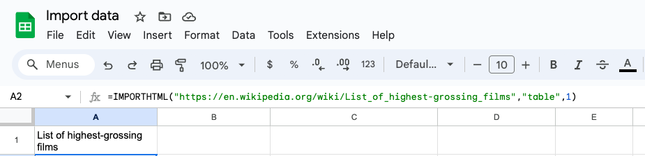
1. Import data straight from a website

When you’re looking to take data — such as from a table or list — from a website and add it to your Google Sheets, you don’t need to go through the hassle of copying and pasting it in yourself.

Instead, use this formula to import the data neatly into columns and rows within the Google Sheet:

=IMPORTHTML(URL)

If there are multiple tables or lists on the website, you’ll need to specify “list” and “1,” or “table” and “2” within the parentheses so Google Sheets can pull in the right data for you. In this case, you’ll also need to put quotation marks around the URL and “list” or “table,” and you’ll need to use a comma between each of the items in the parentheses. Note that the comma should appear outside of the quotation marks.

Here’s how the function will look:

=IMPORTHTML(“URL”, “table/list”, number)

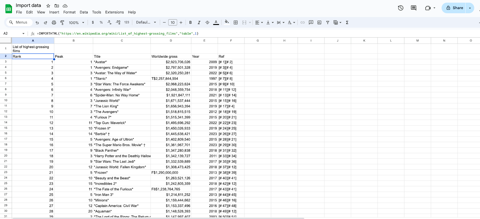
2. Automatically change cell color based on values

In a spreadsheet, it can be hard to get a quick understanding of large quantities of data at a glance. One way to add context to your data is by automatically changing the cell color based on the value that’s in the cell.

For example, in a line item budget, you can highlight every cell with a value over $100 in red, which is a great way to see if you’ve gone over budget on certain items. Similarly, for a task list status check, you can format Google Sheets to turn any cell yellow that includes the word “late.”

Follow these steps to change the cell color based on values:

1. Select the cells for which you want to apply conditional formatting rules.
2. Click Format and then select Conditional formatting.
3. Create a rule in the toolbar that opens up. For example, under “Format cells if…” specify the condition that will initiate a change, such as turning the cell to a specific color.
4. Click Done.

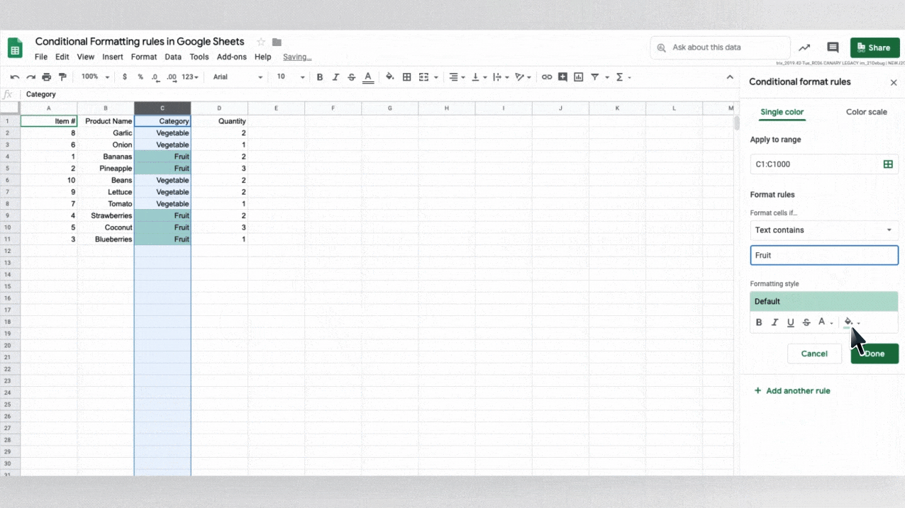
3. Split unorganized data into separate columns

If you’re used to working in spreadsheets, you know how important it is to have data in the right columns and rows. After all, you can’t manage and use the data properly if the spreadsheet is unorganized.

When you have data that requires cleaning and organizing in Google Sheets — such as a column that includes both a name and a date, for example — you can use the SPLIT function to split data into separate columns.

Here’s the SPLIT function formula:

=SPLIT(text, delimiter, [split_by_each], [remove_empty_text])

Apply this to any column with messy data and specify what you need split and removed from that column.

Note: A delimiter is any character or set of characters that identifies the beginning or end of distinct elements in text, code, or a formula.

4. Import an image from the web

While most spreadsheets primarily contain letters and numbers, you can also add images to your Google Sheets.

Of course, you could copy and paste the image from a website. But if you want to use a function that automatically grabs an image from the web and resizes it to fit within your cell, then you need this hack.

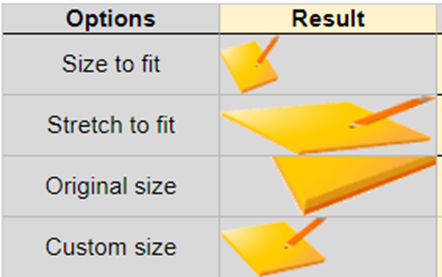
Here’s the IMAGE import function with image sizing options:

• Size to fit: =IMAGE(“URL”), =IMAGE(“URL”, 1)
• Stretch to fit: =IMAGE(“URL”, 2)
• Original size: =IMAGE(“URL”, 3)
• Custom size: =IMAGE(“URL”, 4, [height in pixels], [width in pixels])

5. Create a slicer to view data in different ways

Not everyone likes to view data the same way. To address multiple preferences, you could create different sheets with different views. But it’s simpler to create one sheet with the option for different views embedded in it.

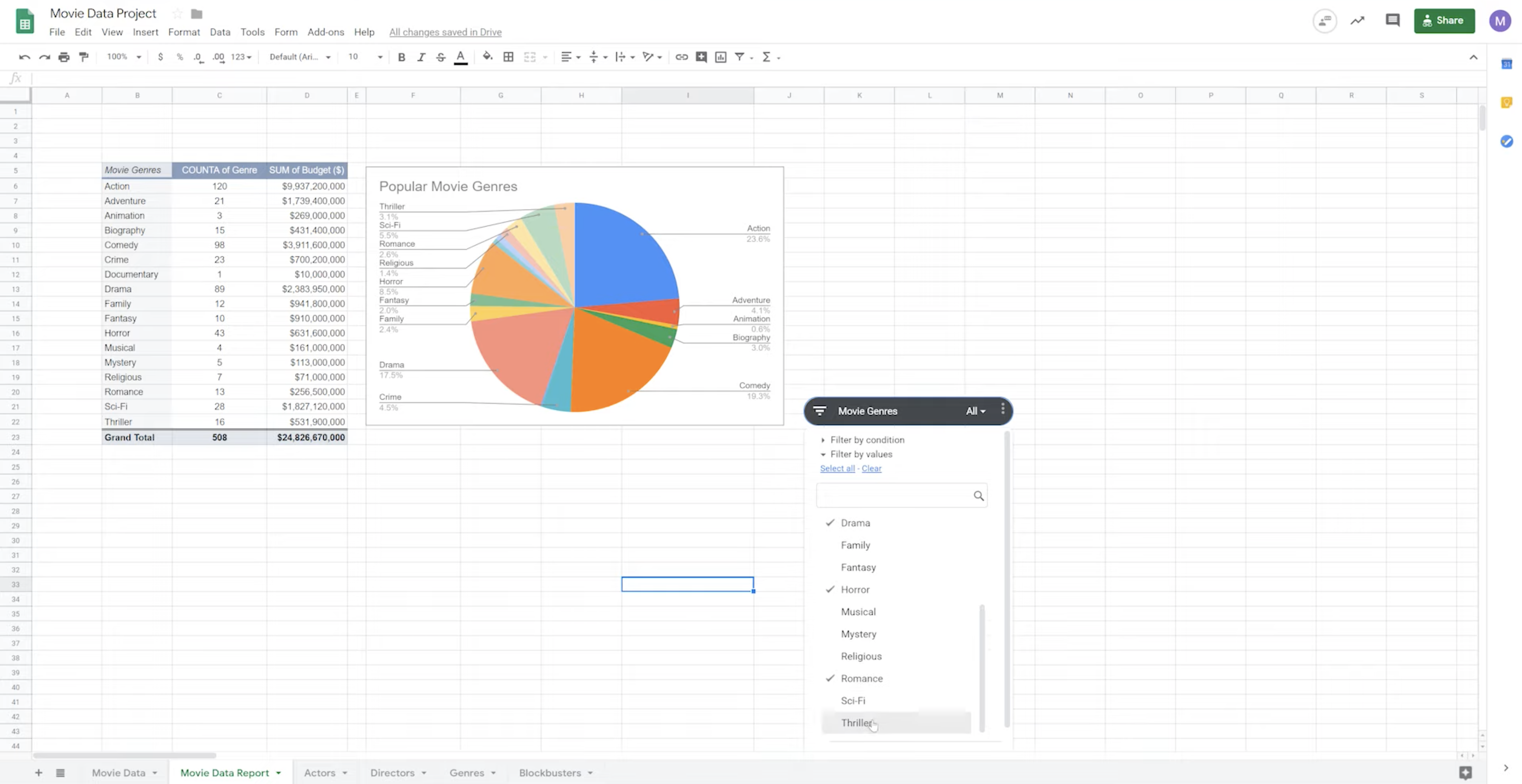
One of the best Google Sheets hacks is to use the slicer functionality, which adds an interactive button to your spreadsheet and gives viewers the ability to “slice” the content in different ways.

Follow these steps to use the slicer functionality:

1. Click on the chart or pivot table you want to filter with the slicer.
2. From the top menu, click Data and then select Add a slicer.
3. Choose a column to filter by .
4. Click the slicer and choose your filter rules. You can choose to filter by condition or by values.

6. Create a dropdown list

Whether you’re making a multiple-choice quiz or an order form, you may want to create dropdown lists in Google Sheets. This not only saves space within the sheet, but it also looks cleaner and more professional.

Follow these steps to create a dropdown list:

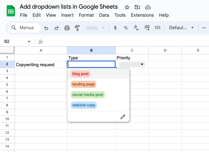
1. Select the cell where you want the dropdown list to appear.
2. Click Data from the top menu and then select Data validation. Click on the + Add rule button.
3. Under Criteria, select Dropdown. In each of the spaces below, type in the items you want in your dropdown list. Click on Add another item if you want more options in your dropdown list.
4. Click Done.

7. Check how a formula works

Formulas are essential for working in Google Sheets. However, there may be times when you know the name of a formula but can’t remember the specific fields within it.

If this happens, you can check the syntax for a formula and get additional details about it within Google Sheets.

Here’s how to learn more about a formula in Google Sheets:

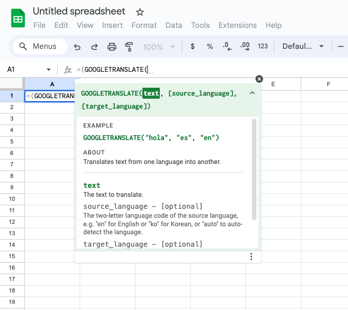
1. Type in a formula you want more information on in any cell.
2. A box with a description of the formula will appear.
3. Click the box to display the elements of the formula and syntax details.

Jotform: For when a simple spreadsheet isn’t enough

Here’s the thing: Google Sheets is a great spreadsheet tool, but sometimes, a spreadsheet just doesn’t cut it. When you’re looking to complete more advanced tasks — such as handling massive data sets — Jotform Tables is a good alternative.

You can connect Jotform forms — including surveys, questionnaires, polls, and more — to Jotform Tables. Assign a form to any table, and your form data will go directly into that table automatically. This way, you can analyze all the data you collect in a powerful database.

You can create a table from scratch, use one of our 300-plus table templates, or import a CSV file. Customize the table to suit your needs — adding formulas, editing data and preferences, adding tags, and so much more — with just a few clicks. Create tabs in different views, such as calendar, cards, or report views, to display your data in the most useful way.

Collaboration is also easy with Jotform Tables. Send your table to collaborators via link or email. You can even add access controls (so the right people have the right type of access) and turn your table into a PDF for sharing and viewing.

The best part? You don’t need any hacks to use Jotform Tables. It’s simple and highly intuitive to use.

Photo by Ilya Pavlov on Unsplash